
SIGNALS:
Systems are classified into the following categories:
- Liner and Non-liner Systems
- Time Variant and Time Invariant Systems
- Liner Time variant and Liner Time invariant systems
- Static and Dynamic Systems
- Causal and Non-causal Systems
- Invertible and Non-Invertible Systems
- Stable and Unstable Systems
Liner and Non-liner Systems
A system is said to be linear when it satisfies superposition and homogenate principles. Consider two systems with inputs as x1(t), x2(t), and outputs as y1(t), y2(t) respectively. Then, according to the superposition and homogenate principles,
T [a1 x1(t) + a2 x2(t)] = a1 T[x1(t)] + a2 T[x2(t)]
∴,∴, T [a1 x1(t) + a2 x2(t)] = a1 y1(t) + a2 y2(t)
From the above expression, is clear that response of overall system is equal to response of individual system.
Example:
(t) = x2(t)
Solution:
y1 (t) = T[x1(t)] = x12(t)
y2 (t) = T[x2(t)] = x22(t)
T [a1 x1(t) + a2 x2(t)] = [ a1 x1(t) + a2 x2(t)]2
Which is not equal to a1 y1(t) + a2 y2(t). Hence the system is said to be non linear.
Time Variant and Time Invariant Systems
A system is said to be time variant if its input and output characteristics vary with time. Otherwise, the system is considered as time invariant.
The condition for time invariant system is:
y (n , t) = y(n-t)
The condition for time variant system is:
y (n , t) ≠≠ y(n-t)
Where y (n , t) = T[x(n-t)] = input change
y (n-t) = output change
Example:
y(n) = x(-n)
y(n, t) = T[x(n-t)] = x(-n-t)
y(n-t) = x(-(n-t)) = x(-n + t)
∴∴ y(n, t) ≠ y(n-t). Hence, the system is time variant.
Liner Time variant (LTV) and Liner Time Invariant (LTI) Systems
If a system is both liner and time variant, then it is called liner time variant (LTV) system.
If a system is both liner and time Invariant then that system is called liner time invariant (LTI) system.
Static and Dynamic Systems
Static system is memory-less whereas dynamic system is a memory system.
Example 1: y(t) = 2 x(t)
For present value t=0, the system output is y(0) = 2x(0). Here, the output is only dependent upon present input. Hence the system is memory less or static.
Example 2: y(t) = 2 x(t) + 3 x(t-3)
For present value t=0, the system output is y(0) = 2x(0) + 3x(-3).
Here x(-3) is past value for the present input for which the system requires memory to get this output. Hence, the system is a dynamic system.
Causal and Non-Causal Systems
A system is said to be causal if its output depends upon present and past inputs, and does not depend upon future input.
For non causal system, the output depends upon future inputs also.
Example 1: y(n) = 2 x(t) + 3 x(t-3)
For present value t=1, the system output is y(1) = 2x(1) + 3x(-2).
Here, the system output only depends upon present and past inputs. Hence, the system is causal.
Example 2: y(n) = 2 x(t) + 3 x(t-3) + 6x(t + 3)
For present value t=1, the system output is y(1) = 2x(1) + 3x(-2) + 6x(4) Here, the system output depends upon future input. Hence the system is non-causal system.
Invertible and Non-Invertible systems
A system is said to invertible if the input of the system appears at the output.
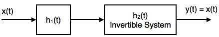
Y(S) = X(S) H1(S) H2(S)
= X(S) H1(S) · 1(H1(S))1(H1(S)) Since H2(S) = 1/( H1(S) )
∴,∴, Y(S) = X(S)
→→ y(t) = x(t)
Hence, the system is invertible.
If y(t) ≠≠ x(t), then the system is said to be non-invertible.
Stable and Unstable Systems
The system is said to be stable only when the output is bounded for bounded input. For a bounded input, if the output is unbounded in the system then it is said to be unstable.
Note: For a bounded signal, amplitude is finite.
Example 1: y (t) = x2(t)
Let the input is u(t) (unit step bounded input) then the output y(t) = u2(t) = u(t) = bounded output.
Hence, the system is stable.
Example 2: y (t) = ∫x(t)dt∫x(t)dt
Let the input is u (t) (unit step bounded input) then the output y(t) = ∫u(t)dt∫u(t)dt= ramp signal (unbounded because amplitude of ramp is not finite it goes to infinite when t →→ infinite).
Hence, the system is unstable.
LAPLACE TRANSFORMATION
The Laplace transform is a frequency-domain approach for continuous time signals irrespective of whether the system is stable or unstable. The Laplace transform of a functions f(t), defined for all real numbers t ≥ 0, is the function F(s), which is a unilateral transform defined by

where s is a complex number frequency parameter
-
, with real numbers σ and ω.
Other notations for the Laplace transform include L{f} , or alternatively L{f(t)} instead of F.
The meaning of the integral depends on types of functions of interest. A necessary condition for existence of the integral is that f must be locally integrable on [0, ∞). For locally integrable functions that decay at infinity or are of exponential type, the integral can be understood to be a (proper) Lebesgue integral. However, for many applications it is necessary to regard it to be a conditionally convergent improper integral at ∞. Still more generally, the integral can be understood in a weak sense, and this is dealt with below.
One can define the Laplace transform of a finite Borel measure μ by the Lebesgue integral

An important special case is where μ is a probability measure, for example, the Dirac delta function. In operational calculus, the Laplace transform of a measure is often treated as though the measure came from a probability density function f. In that case, to avoid potential confusion, one often writes

where the lower limit of 0− is shorthand notation for

This limit emphasizes that any point mass located at 0 is entirely captured by the Laplace transform. Although with the Lebesgue integral, it is not necessary to take such a limit, it does appear more naturally in connection with the Laplace–Stieltjes transform.
Z-TRANSFORM
Definition
The Z-transform can be defined as either a one-sided or two-sided transform.
Bilateral Z-transform
The bilateral or two-sided Z-transform of a discrete-time signal x[n] is the formal power series X(z) defined as
![X(z)={\mathcal {Z}}\{x[n]\}=\sum _{n=-\infty }^{\infty }x[n]z^{-n}](https://wikimedia.org/api/rest_v1/media/math/render/svg/12f6e27003f8c3271124b8af3ea0092c2906ae3e)
where n is an integer and z is, in general, a complex number:

where A is the magnitude of z, j is the imaginary unit, and ɸ is the complex argument (also referred to as angle or phase) in radians.
Unilateral Z-transform
Alternatively, in cases where x[n] is defined only for n ≥ 0, the single-sided or unilateral Z-transform is defined as
![X(z)={\mathcal {Z}}\{x[n]\}=\sum _{n=0}^{\infty }x[n]z^{-n}.](https://wikimedia.org/api/rest_v1/media/math/render/svg/a3e560ddcffcbab6fa176f4d2dd8e3fe60905b55)
In signal processing, this definition can be used to evaluate the Z-transform of the unit impulse response of a discrete-time causal system.
An important example of the unilateral Z-transform is the probability-generating function, where the component x[n] is the probability that a discrete random variable takes the value n, and the function X(z) is usually written as X(s), in terms of s = z−1. The properties of Z-transforms (below) have useful interpretations in the context of probability theory.
Geophysical definition
In geophysics, the usual definition for the Z-transform is a power series in z as opposed to z−1. This convention is used, for example, by Robinson and Treitel and by Kanasewich The geophysical definition is:
-
-
FOURIER SERIES AND ITS PROPERTIRES:
Fourier series
Fourier transform refers to the transform of functions of a continuous real argument, and it produces a continuous function of frequency, known as a frequency distribution. One function is transformed into another, and the operation is reversible. When the domain of the input (initial) function is time (t), and the domain of the output (final) function is ordinary frequency, the transform of function s(t) at frequency f is given by the complex number:
Evaluating this quantity for all values of f produces the frequency-domain function. Then s(t) can be represented as a recombination of complex exponentials of all possible frequencies:
which is the inverse transform formula. The complex number, S( f ), conveys both amplitude and phase of frequency f.
See Fourier transform for much more information, including:
- conventions for amplitude normalization and frequency scaling/units
- transform properties
- tabulated transforms of specific functions
- an extension/generalization for functions of multiple dimensions, such as images.
Fourier series
The Fourier transform of a periodic function, sP(t), with period P, becomes a Dirac comb function, modulated by a sequence of complex coefficients:
for all integer values of k, and where ∫P is the integral over any interval of length P.
The inverse transform, known as Fourier series, is a representation of sP(t) in terms of a summation of a potentially infinite number of harmonically related sinusoids or complex exponential functions, each with an amplitude and phase specified by one of the coefficients:
When sP(t), is expressed as a periodic summation of another function, s(t):
the coefficients are proportional to samples of S( f ) at discrete intervals of 1/P:
A sufficient condition for recovering s(t) (and therefore S( f )) from just these samples is that the non-zero portion of s(t) be confined to a known interval of duration P, which is the frequency domain dual of the Nyquist–Shannon sampling theorem.
See Fourier series for more information, including the historical development.
Discrete-time Fourier transform (DTFT)
a convergent periodic summation in the frequency domain can be represented by a Fourier series, whose coefficients are samples of a related continuous time function:
The Fourier series coefficients (and inverse transform), are defined by:
These are properties of Fourier series:
Linearity Property
Time Shifting Property
Frequency Shifting Property
Time Reversal Property
Time Scaling Property
Differentiation and Integration Properties
Multiplication and Convolution Properties
Conjugate and Conjugate Symmetry Properties
-
![X(z)={\mathcal {Z}}\{x[n]\}=\sum _{n}x[n]z^{n}.](https://wikimedia.org/api/rest_v1/media/math/render/svg/af64bf848f2f92b8aab0469ae4c87827d8092916)


![{\displaystyle S[k]={\frac {1}{P}}\int _{P}s_{P}(t)\cdot e^{-2i\pi {\frac {k}{P}}t}\,dt}](https://wikimedia.org/api/rest_v1/media/math/render/svg/3f81650bdeebd32083db91537bd202f5c172b5cf)
![{\displaystyle s_{P}(t)=\sum _{k=-\infty }^{\infty }S[k]\cdot e^{2i\pi {\frac {k}{P}}t}\quad {\stackrel {\displaystyle {\mathcal {F}}}{\Longleftrightarrow }}\quad \sum _{k=-\infty }^{+\infty }S[k]\,\delta \left(f-{\frac {k}{P}}\right).}](https://wikimedia.org/api/rest_v1/media/math/render/svg/d11b0c1739829986923c0c552620bbfd3ecadcb0)

![{\displaystyle S[k]={\frac {1}{P}}\cdot S\left({\frac {k}{P}}\right).}](https://wikimedia.org/api/rest_v1/media/math/render/svg/639522ac155d3a2aa8c2fcf1a47a69a699f0a0c2)
![{\displaystyle S_{\frac {1}{T}}(f)\ {\stackrel {\text{def}}{=}}\ \underbrace {\sum _{k=-\infty }^{\infty }S\left(f-{\frac {k}{T}}\right)\equiv \overbrace {\sum _{n=-\infty }^{\infty }s[n]\cdot e^{-2i\pi fnT}} ^{\text{Fourier series (DTFT)}}} _{\text{Poisson summation formula}}={\mathcal {F}}\left\{\sum _{n=-\infty }^{\infty }s[n]\ \delta (t-nT)\right\},\,}](https://wikimedia.org/api/rest_v1/media/math/render/svg/a8e6c7cd8298d83f92f03842f193b1515a19e350)
![{\displaystyle s[n]\ {\stackrel {\mathrm {def} }{=}}\ T\int _{\frac {1}{T}}S_{\frac {1}{T}}(f)\cdot e^{2i\pi fnT}\,df=T\underbrace {\int _{-\infty }^{\infty }S(f)\cdot e^{2i\pi fnT}\,df} _{{\stackrel {\mathrm {def} }{=}}\,s(nT)}}](https://wikimedia.org/api/rest_v1/media/math/render/svg/189510781f106b706581248689361a54e856f355)
