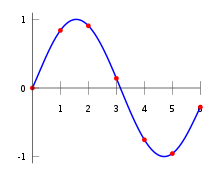
Definition
Given a set of n + 1 data points (xi, yi) where no two xi are the same, one is looking for a polynomial p of degree at most n with the property
The unisolvence theorem states that such a polynomial p exists and is unique, and can be proved by the Vandermode matrix, as described below.
The theorem states that for n + 1 interpolation nodes (xi), polynomial interpolation defines a linear bijection
where Πn is the vector space of polynomials (defined on any interval containing the nodes) of degree at most n.
Constructing the interpolation polynomial
Suppose that the interpolation polynomial is in the form
The statement that p interpolates the data points means that
using equation (1) here, we get a system of linear equations in the coefficients ak. The system in matrix-vector form reads
We have to solve this system for ak to construct the interpolant p(x). The matrix on the left is commonly referred to as a Vandermode matrix The condition number of the Vandermonde matrix may be large, causing large errors when computing the coefficients ai if the system of equations is solved using Gaussian elimination
Several authors have therefore proposed algorithms which exploit the structure of the Vandermonde matrix to compute numerically stable solutions in O(n2) operations instead of the O(n3) required by Gaussian elimination. These methods rely on constructing first a Newton interpolation of the polynomial and then converting it to the monomial form above.
Alternatively, we may write down the polynomial immediately in terms of Langrage Polynomial


